Vanilla RNN’s are overviewed in detail in quite a few works of machine learning literature. However, I find that some of the intricate details to be a lacking. Particularly with what happens with layers surrounding the RNN layer. Furthermore when I first started I had questions like :

• Do we need to iterate all layers backprop_interval times?
• Does every layer need to hold a list of inputs / outputs for each backprop_interval?
• Do we need backprop_interval number of weights for the RNN layer?
• Do we need to cache all the state derivatives of the RNN layer?

For this reason we will work through the backprop-through-time equations for an RNN with a prior and post ANN layer and see how we can cache/reuse certain parameters.

Forward Propagation

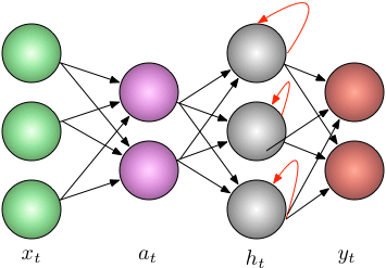
It’s always best to start off defining what each variable means and assume a sample sizing.
This ensures that we get our dimensions right along the way.

Variable Definition	Assumed Sizing
$x_t$: input at time t	[128 x 10]
$a_t^0$: $ANN_0$ activation at time t	[128 x 20]
$h_t$: rnn output at time t	[128 x 5]
$W_{x_t}^T, W_{h_t}^T, W_{y_t}^T$: Weights for $ANN_0$, RNN and $ANN_1$	[10 x 20] , [20 x 5], [5 x 100]
$U_{h_t}^T$: Recurrent weights at time t	[5 x 5]
$b_{x_t}, b_{h_t}, b_{y_t}$: Biases for $ANN_0$, RNN and $ANN_1$	[20], [5], [100]
$\sigma_{0,1,2}$: Activation of first, second and third layers	[128 x 20], [128 x 5], [128 x 100]
$\sigma_{0,1,2}^\prime$: Derivative of the activation of first, second and third layers	[128 x 20], [128 x 5], [128 x 100]
$\hat{y_t}$: prediction at time t	[128, 100]

$$\begin{aligned} a_t^0 &= \sigma_0(x_tW_{x_t}^T + b_{x_t}) \\ h_t &= \sigma_1(a_t^0W_{h_t}^T + h_{t-1}U_{h_t}^T + b_{h_t}) \\ \hat{y}_t &= \sigma_2(h_tW_{y_t}^T + b_{y_t}) \\ \mathcal{L} &= f(\hat{y}_t, y_t) \end{aligned}$$

We leave the loss $\mathcal{L}$ to be arbitrary for generalization purposes. An example loss could be an L2 loss for regression or perhaps a cross-entropy loss for classification. We leave the sizing in transpose-weight notation because it keeps logic consistent with data being in the shape of [batch_size, feature]

Backpropagation Through Time

The chain rule for the final ANN [i.e. the emitter of $\hat{y}_t$]:

$$\begin{aligned} \frac{\delta\mathcal{L}}{\delta W_{y_t}} &= \frac{\delta \mathcal{L}}{\delta \hat{y}_t} \frac{\delta\hat{y}_t}{\delta W_{y_t}} = [\delta_t^{Loss}\odot\sigma_2^\prime(h_tW_{y_t}^T + b_{y_t})]^Th_t \ \ = [\delta_t^{Loss}\odot\sigma_2^\prime(z_{y_t})]^T h_t \\ \frac{\delta\mathcal{L}}{\delta b_{y_t}} &= \frac{\delta\mathcal{L}}{\delta\hat{y}_t} \frac{\delta\hat{y}_t} {\delta b_{y_t}} = \sum_{batch}[\delta_t^{Loss}\odot\sigma_2^\prime(h_tW_{y_t}^T + b_{y_t})] = \sum_{batch}[\delta_t^{Loss}\odot\sigma_2^\prime(z_{y_t})] \end{aligned}$$

Note that $\delta_t^{Loss}$ is merely the loss derivative. For an L2 loss this is just $(\hat{y}_t - y)$.
We then pass the following $\delta_t^{L-1}$ back to the previous RNN layer:

$$\begin{aligned} \delta_t^{L-1} &= \frac{\delta\mathcal{L}}{\delta\hat{y}_t} \frac{\delta\hat{y}_t}{\delta h_t} = [\delta_t^{Loss}\odot\sigma_2^\prime(z_{y_t})]W_{y_t} \end{aligned}$$

The chain rule for the RNN:

A key point that makes the RNN different from a standard ANN is that the derivative of the hidden state is sent backwards through time and compounded through a simple addition operation. More formally this means:

$$\begin{aligned} \frac{\delta h_t}{\delta h_{t-1}} &= \sigma_1^\prime(a_t^0W_{h_t}^T + h_{t-1}U_{h_t}^T + b_{h_t}) U_{h_t} \ = \sigma_1^\prime(z_{h_t}) U_{h_t} \end{aligned}$$

This value is sent backwards through time from the final BPTT time step ($T_f$ below) until till time t=0. In computation terms this means that $\frac{\delta {h_t}}{\delta h_{t-1}}$ needs to be cached and added to itself. Listed below is an example of two time steps of accumulation of the hidden state:

$$\begin{aligned} \Delta h_{T_f} &= \frac{\delta h_{T_f}}{\delta h_{T_{f-1}}} \\ \Delta h_{T_{f-1}} &= \Delta h_{T_f} + \frac{\delta h_{T_{f-1}}}{\delta h_{T_{f-2}}} \end{aligned}$$

This process is repeated up till the last unroll after which the hidden state’s derivative accumulator is zero’d out (you can also do this when you zero out the gradients in the optimizer).

$$\begin{aligned} \frac{\delta\mathcal{L}}{\delta W_{h_t}} &= \frac{\delta \mathcal{L}}{\delta \hat{y}_t} \frac{\delta\hat{y}_t}{\delta h_t} \frac{\delta h_t}{\delta W_{h_t}} = [(\delta_t^{L-1} + \Delta h_t)\odot\sigma_1^\prime(a_t^0W_{h_t}^T + h_{t-1}U_{h_t}^T + b_{h_t})]^Ta_t^0 \ \ \ = [(\delta_t^{L-1} + \Delta h_t)\odot\sigma_1^\prime(z_{h_{t}})]^Ta_t^0 \\ \frac{\delta\mathcal{L}}{\delta U_{h_t}} &= \frac{\delta \mathcal{L}}{\delta \hat{y}_t} \frac{\delta\hat{y}_t}{\delta h_t} \frac{\delta h_t}{\delta U_{h_t}} = [(\delta_t^{L-1} + \Delta h_t)\odot\sigma_1^\prime(a_t^0W_{h_t}^T + h_{t-1}U_{h_t}^T + b_{h_t})]^Th_{t-1} = [(\delta_t^{L-1} + \Delta h_t)\odot\sigma_1^\prime(z_{h_{t}})]^Th_{t-1} \\ \frac{\delta\mathcal{L}}{\delta b_{h_t}} &= \frac{\delta \mathcal{L}}{\delta \hat{y}_t} \frac{\delta\hat{y}_t}{\delta h_t} \frac{\delta h_t}{\delta b_{h_t}} = \sum_{batch}[(\delta_t^{L-1} + \Delta h_t)\odot\sigma_1^\prime(a_t^0W_{h_t}^T + h_{t-1}U_{h_t}^T + b_{h_t})] \ \ \ = \sum_{batch}[(\delta_t^{L-1} + \Delta h_t)\odot\sigma_1^\prime(z_{h_{t}})] \end{aligned}$$

As shown above we have that all the parameters of the RNN depend on $h_{t-1}$ and that is defined as:

$$\begin{aligned} h_{t-1} &= \sigma_1(a_{t-1}^0W_{h_{t-1}}^T + h_{t-2}U_{h_{t-1}}^T + b_{h_{t-1}}) \\ \end{aligned}$$

An insight here is that the parameters are shared across time; we don’t in fact use different parameters for the RNN, but merely share and jointly update them using BPTT. So with this little tidbit of knowledge we can rewrite our equation from above as such :

$$\begin{aligned} h_{t-1} &= \sigma_1(a_{t-1}^0W_{h_t}^T + h_{t-2}U_{h_t}^T + b_{h_{t}}) \\ \end{aligned}$$

This leaves us with the following unsatisfied requirement: $a_{t-1}^0$ which is the activated response from the first ANN. Before we sort out the logistics of the entire BPTT algorithm let’s just write out the equations for the first layer.

The RNN layer will emit $\delta_t^{L-2}$ which will be used to update the parameters of the first ANN.

$$\begin{aligned} \delta_t^{L-2} &= \frac{\delta\mathcal{L}}{\delta\hat{y}_t} \frac{\delta\hat{y}_t}{\delta h_t} \frac{\delta h_t}{\delta a_t^0} = [(\delta_t^{L-1} + \Delta h_t)\odot\sigma_1^\prime(z_{h_t})]W_{h_t} \\ \end{aligned}$$

The chain rule for the first ANN [i.e. the emitter of $a_t^0$]:

$$\begin{aligned} \frac{\delta\mathcal{L}}{\delta W_{x_t}} &= \frac{\delta \mathcal{L}}{\delta \hat{y}_t} \frac{\delta\hat{y}_t}{\delta h_t} \frac{\delta h_t}{\delta a_t^0} \frac{\delta a_t^0}{\delta W_{x_t}} = [\delta_t^{L-2}\odot\sigma_0^\prime(x_t W_{x_t}^T + b_{x_t})]^T x_t = [\delta_t^{L-2} \odot \sigma_0^\prime(z_{x_t})]^T x_t \\ \frac{\delta\mathcal{L}}{\delta b_{x_t}} &= \frac{\delta \mathcal{L}}{\delta \hat{y}_t} \frac{\delta\hat{y}_t}{\delta h_t} \frac{\delta h_t}{\delta a_t^0} \frac{\delta a_t^0}{\delta b_{x_t}} = \sum_{batch}[\delta_t^{L-2}\odot\sigma_0^\prime(x_t W_{x_t}^T + b_{x_t})] = \sum_{batch}[\delta_t^{L-2} \odot \sigma_0^\prime(z_{x_t})] \end{aligned}$$

Sizing Verification:

Before we move on let’s just verify that the size of the following are the same.
This is left as an exercise to the reader.

Variable Name	Desired Size
$\frac{\delta\mathcal{L}}{\delta W_{y_t}^T}$ : derivative of $ANN_1$’s weight matrix	[5 x 100]
$\frac{\delta\mathcal{L}}{\delta b_{y_t}}$ : derivative of $ANN_1$’s bias vector	[100]
$\frac{\delta\mathcal{L}}{\delta W_{h_t}^T}$ : derivative of RNN input-to-hidden weight matrix	[20 x 5]
$\frac{\delta\mathcal{L}}{\delta U_{h_t}^T}$ : derivative of the RNN’s recurrent weight matrix	[5 x 5]
$\frac{\delta\mathcal{L}}{\delta b_{h_t}}$ : derivative of the RNN’s bias vector	[5]
$\frac{\delta\mathcal{L}}{\delta W_{x_t}^T}$ : derivative of $ANN_0$’s weight matrix	[10 x 20]
$\frac{\delta\mathcal{L}}{\delta b_{x_t}}$ : derivative of $ANN_0$’s bias vector	[20]
$\delta_t^{Loss}$ : loss delta	[128 x 100]
$\delta_t^{L-1}$ : delta from $ANN_1$ to RNN	[128 x 5]
$\delta_t^{L-2}$ : delta from RNN to $ANN_0$	[128 x 20]

Step-by-step Forward / Backward Procedure:

Let’s think about this from another way: let’s start by writing the above equations from $t=0$.
In the example below we will walk through three time steps [i.e our BPTT interval is 3]:

1. We start off by initializing the first hidden layer to be zero since we have no data up to this point.
2. We can then use $h_{-1}$ and the new $x_0$ to calculate $a_0$, $h_0$, $\hat{y}_0$ and finally $L_0$
3. We repeat this (i.e. we pass the h from the current time to the next time step) and do this for the BPTT interval.

It is good to note here that each of these are vectors. While the loss in the end is reduced via a sum / mean to a single number, for the purposes of backpropagation it is still a vector (eg: $[\hat{y} - y]$).

The backward pass is shown above. The key here is that you just update one time slice at a time in the same way you would in a classical neural network. So to revisit the questions posed earlier:

• Do we need to iterate all layers backprop_interval times? Yes, you need to get all the loss vectors for the corresponding input minibatches (at each timestep).
• Does every layer need to hold a list of inputs / outputs for each backprop_interval? Yes. SGD updates are only done after backprop_interval forward pass operations. Since this is the case each layer will need to hold the input / output mapping for each one of those forward passes. This is what makes an RNN trained with backprop-through-time memory intensive as the memory scales with the length of the BPTT interval.
• Do we need backprop_interval number of weights for the RNN layer? No! They are shared weights/biases between all the recurrent layers and they are updated in one fail swoop!
• Do we need to cache all the state derivatives of the RNN layer? No! Since they are compounded via a simple addition operator you merely need to keep one value and recursively add to it.

Issues

If you find any errors with any of the math or logic here please leave a comment below.

comments powered by Disqus